Using the OpenAQ API
The openaq api is an easy-to-use wrapper built around the OpenAQ
Api. Complete API documentation can be
found on their website.
There are no keys or rate limits (as of March 2017), so working with the
API is straight forward. If building a website or app, you may want to
just use the python wrapper and interact with the data in json format.
However, the rest of this tutorial will assume you are interested in
analyzing the data. To get more out of it, I recommend installing
seaborn for manipulating the asthetics of plots, and working with
data as DataFrames using pandas. For more information on these,
check out the installation section of this documentation.
From this point forward, I assume you have at least a basic knowledge of python and matplotlib. This documentation was built using the following versions of all packages:
import pandas as pd
import seaborn as sns
import matplotlib as mpl
import matplotlib.pyplot as plt
import openaq
import warnings

warnings.simplefilter('ignore')

%matplotlib inline

# Set major seaborn asthetics
sns.set("notebook", style='ticks', font_scale=1.0)

# Increase the quality of inline plots
mpl.rcParams['figure.dpi']= 500

print ("pandas v{}".format(pd.__version__))
print ("matplotlib v{}".format(mpl.__version__))
print ("seaborn v{}".format(sns.__version__))
print ("openaq v{}".format(openaq.__version__))
pandas v0.21.0
matplotlib v2.1.0
seaborn v0.8.1
openaq v1.1.0
OpenAQ API
The OpenAQ APi has only eight endpoints that we are interested in:
- cities: provides a simple listing of cities within the platforms
- countries: provides a simple listing of countries within the platform
- fetches: providing data about individual fetch operations that are used to populate data in the platform
- latest: provides the latest value of each available parameter for every location in the system
- locations: provides a list of measurement locations and their meta data
- measurements: provides data about individual measurements
- parameters: provides a simple listing of parameters within the platform
- sources: provides a list of data sources
For detailed documentation about each one in the context of this API wrapper, please check out the API documentation.
Your First Request
Real quick, let’s go ahead and initiate an instance of the
openaq.OpenAQ class so we can begin looking at data:
api = openaq.OpenAQ()
Cities
The cities API endpoint lists the cities available within the platform. Results can be subselected by country and paginated to retrieve all results in the database. Let’s start by performing a basic query with an increased limit (so we can get all of them) and return it as a DataFrame:
resp = api.cities(df=True, limit=10000)

# display the first 10 rows
resp.info()
<class 'pandas.core.frame.DataFrame'>
RangeIndex: 2020 entries, 0 to 2019
Data columns (total 4 columns):
city         2020 non-null object
count        2020 non-null int64
country      2020 non-null object
locations    2020 non-null int64
dtypes: int64(2), object(2)
memory usage: 63.2+ KB
So we retrieved 1400+ entries from the database. We can then take a look at them:
print (resp.head(10))
                                           city   count country  locations
0                            Escaldes-Engordany   13324      AD          2
1                                        unused     314      AD          1
2                                     Abu Dhabi     477      AE          1
3                                  Buenos Aires   14976      AR          4
4              Amt der K�rntner Landesregierung  104663      AT         16
5                                       Austria  121987      AT        174
6  Amt der Ober�sterreichischen Landesregierung  154329      AT         16
7      Amt der Burgenl�ndischen Landesregierung   35608      AT          3
8            Amt der Salzburger Landesregierung   94197      AT         12
9      Amt der Burgenländischen Landesregierung     471      AT          1
Let’s try to find out which ones are in India:
print (resp.query("country == 'IN'"))
                   city    count country  locations
841              Mumbai   309477      IN          3
842                Kota    23264      IN          2
843               Delhi  1140259      IN         35
844           Ghaziabad    99087      IN          2
845          Barddhaman     2470      IN          3
846             Asansol     1590      IN          2
847             Lucknow   271912      IN          5
848         Muzaffarpur   116841      IN          1
849           Hyderabad   465962      IN         15
850       Visakhapatnam   208237      IN          8
851            Amritsar    77849      IN          1
852             Bhiwadi    20846      IN          1
853             Kolkata   168542      IN          7
854           Bengaluru   371649      IN          8
855              Howrah    50263      IN          4
856         Navi Mumbai     7725      IN          1
857           Ahmedabad    57714      IN          2
858           Faridabad   113546      IN          2
859              Nashik    76217      IN          4
860              Haldia   115284      IN          2
861  Thiruvananthapuram    46124      IN          2
862              Rohtak    95050      IN          1
863               Medak     2671      IN          1
864                Pune   145450      IN          1
865            Tirupati   159117      IN          4
866               Ajmer    25266      IN          2
867          Vijayawara    34902      IN          1
868            Durgapur    78761      IN          2
869          Jorapokhar    35558      IN          1
870               NOIDA    12061      IN          1
..                  ...      ...     ...        ...
873                Gaya    76810      IN          1
874          Chandrapur   232244      IN          2
875             Chennai   290415      IN          4
876            Siliguri       30      IN          2
877               Thane   130025      IN          3
878              Nagpur    72328      IN          5
879           Mandideep     7847      IN          1
880               Patna    75338      IN          1
881             Dhanbad        3      IN          1
882          Aurangabad   113529      IN          1
883              Kanpur   159678      IN          2
884           Moradabad    24595      IN          1
885            Chittoor     2013      IN          1
886               Alwar    14017      IN          1
887          Vijayawada    11624      IN          2
888             Udaipur    25699      IN          1
889              Jaipur   190441      IN          6
890            Ludhiana    72308      IN          1
891            Varanasi   181673      IN          1
892                Pali    23627      IN          2
893              Ujjain    16924      IN          1
894           Singrauli    14636      IN          1
895             Jodhpur   151172      IN          1
896                Agra    84301      IN          1
897               Dewas    11671      IN          1
898           Amaravati    11432      IN          1
899    Mandi Gobindgarh    48579      IN          1
900             Solapur   253940      IN          1
901           Pithampur    12173      IN          1
902             Gurgaon   147910      IN          1

[62 rows x 4 columns]
Great! For the rest of the tutorial, we are going to focus on Delhi, India. Why? Well..because there are over 500,000 data points and my personal research is primarily in India. We will also take a look at some \(SO_2\) data from Hawai’i later on (another great research locale).
Countries
Similar to the cities endpoint, the countries endpoint lists the
countries available. The only parameters we have to play with are the
limit and page number. If we want to grab them all, we can just up the
limit to the maximum (10000).
res = api.countries(limit=10000, df=True)

print (res.head())
   cities code    count  locations       name
0       2   AD    13638          3    Andorra
1       1   AR    14976          4  Argentina
2      18   AU  3248142         99  Australia
3      16   AT  1521351        306    Austria
4       1   BH    13820          1    Bahrain
Fetches
If you are interested in getting information pertaining to the
individual data fetch operations, go ahead and use this endpoint. Most
people won’t need to use this. This API method does not allow the df
parameter; if you would like it to be added, drop me a message.
Otherwise, here is how you can access the json-formatted data:
status, resp = api.fetches(limit=1)

# Print out the meta info
resp['meta']
{'found': 92506,
 'license': 'CC BY 4.0',
 'limit': 1,
 'name': 'openaq-api',
 'page': 1,
 'pages': 92506,
 'website': 'https://docs.openaq.org/'}
Parameters
The parameters endpoint will provide a listing off all the
parameters available:
res = api.parameters(df=True)

print (res)
                                         description    id   name  0                                       Black Carbon    bc     BC
1                                    Carbon Monoxide    co     CO
2                                   Nitrogen Dioxide   no2    NO2
3                                              Ozone    o3     O3
4  Particulate matter less than 10 micrometers in...  pm10   PM10
5  Particulate matter less than 2.5 micrometers i...  pm25  PM2.5
6                                     Sulfur Dioxide   so2    SO2

  preferredUnit
0         µg/m³
1           ppm
2           ppm
3           ppm
4         µg/m³
5         µg/m³
6           ppm
Sources
The sources endpoint will provide a list of the sources where the
raw data came from.
res = api.sources(df=True)

# Print out the first one
res.ix[0]
active                                                       True
adapter                                                 arpalazio
city                                                          NaN
contacts                                        [info@openaq.org]
country                                                        IT
description             Air quality data from Lazio region, Italy
location                                                      NaN
name                                                    ARPALAZIO
organization                                                  NaN
region                                                      Lazio
resolution                                                    NaN
sourceURL                               http://www.arpalazio.net/
timezone                                                      NaN
url             http://www.arpalazio.net/main/aria/sci/annoinc...
Name: 0, dtype: object
Locations
The locations endpoint will return the list of measurement locations
and their meta data. We can do quite a bit of querying with this one:
Let’s see what the data looks like:
res = api.locations(df=True)

res.info()
<class 'pandas.core.frame.DataFrame'>
RangeIndex: 100 entries, 0 to 99
Data columns (total 11 columns):
city                     100 non-null object
coordinates.latitude     100 non-null float64
coordinates.longitude    100 non-null float64
count                    100 non-null int64
country                  100 non-null object
firstUpdated             100 non-null datetime64[ns]
lastUpdated              100 non-null datetime64[ns]
location                 100 non-null object
parameters               100 non-null object
sourceName               100 non-null object
sourceNames              100 non-null object
dtypes: datetime64[ns](2), float64(2), int64(1), object(6)
memory usage: 8.7+ KB
# print out the first one
res.ix[0]
city                                  Ulaanbaatar
coordinates.latitude                      47.9329
coordinates.longitude                     106.921
count                                      294682
country                                        MN
firstUpdated                  2015-09-01 00:00:00
lastUpdated                   2018-01-24 13:15:00
location                                  100 ail
parameters               [pm10, no2, so2, o3, co]
sourceName                               Agaar.mn
sourceNames                            [Agaar.mn]
Name: 0, dtype: object
What if we just want to grab the locations in Delhi?
res = api.locations(city='Delhi', df=True)


res.ix[0]
city                                              Delhi
coordinates.latitude                            28.6508
coordinates.longitude                           77.3152
count                                            102326
country                                              IN
distance                                    6.32199e+06
firstUpdated                        2015-06-29 14:30:00
lastUpdated                         2017-11-28 10:15:00
location                                    Anand Vihar
parameters               [pm10, pm25, so2, o3, co, no2]
sourceName                                         CPCB
sourceNames                         [Anand Vihar, CPCB]
Name: 0, dtype: object
What about just figuring out which locations in Delhi have \(PM_{2.5}\) data?
res = api.locations(city='Delhi', parameter='pm25', df=True)

res.ix[0]
city                                   Delhi
coordinates.latitude                 28.6508
coordinates.longitude                77.3152
count                                  23891
country                                   IN
firstUpdated             2015-06-29 14:30:00
lastUpdated              2017-11-28 10:15:00
location                         Anand Vihar
parameters                            [pm25]
sourceName                              CPCB
sourceNames              [CPCB, Anand Vihar]
Name: 0, dtype: object
Latest
Grab the latest data from a location or locations.
What was the most recent \(PM_{2.5}\) data in Delhi?
res = api.latest(city='Delhi', parameter='pm25', df=True)

res.head()
| averagingPeriod.unit | averagingPeriod.value | city | country | location | parameter | sourceName | unit | value | |
|---|---|---|---|---|---|---|---|---|---|
| lastUpdated | |||||||||
| 2017-11-28 10:15:00 | hours | 0.25 | Delhi | IN | Anand Vihar | pm25 | CPCB | b'\xc2\xb5g/m\xc2\xb3' | 70.00 |
| 2018-01-24 09:45:00 | hours | 0.25 | Delhi | IN | Anand Vihar, Delhi - DPCC | pm25 | CPCB | b'\xc2\xb5g/m\xc2\xb3' | 160.00 |
| 2018-01-24 01:15:00 | hours | 0.25 | Delhi | IN | Aya Nagar, Delhi - IMD | pm25 | CPCB | b'\xc2\xb5g/m\xc2\xb3' | 192.84 |
| 2018-01-24 01:15:00 | hours | 0.25 | Delhi | IN | Burari Crossing, Delhi - IMD | pm25 | CPCB | b'\xc2\xb5g/m\xc2\xb3' | 53.45 |
| 2018-01-24 01:15:00 | hours | 0.25 | Delhi | IN | CRRI Mathura Road, Delhi - IMD | pm25 | CPCB | b'\xc2\xb5g/m\xc2\xb3' | 185.60 |
What about the most recent \(SO_2\) data in Hawii?
res = api.latest(city='Hilo', parameter='so2', df=True)

res
| averagingPeriod.unit | averagingPeriod.value | city | country | location | parameter | sourceName | unit | value | |
|---|---|---|---|---|---|---|---|---|---|
| lastUpdated | |||||||||
| 2018-01-24 06:00:00 | hours | 1 | Hilo | US | Hawaii Volcanoes NP | so2 | AirNow | ppm | 0.000 |
| 2018-01-24 06:00:00 | hours | 1 | Hilo | US | Hilo | so2 | AirNow | ppm | 0.001 |
| 2018-01-24 06:00:00 | hours | 1 | Hilo | US | Kona | so2 | AirNow | ppm | 0.003 |
| 2018-01-24 06:00:00 | hours | 1 | Hilo | US | Ocean View | so2 | AirNow | ppm | 0.002 |
| 2018-01-24 06:00:00 | hours | 1 | Hilo | US | Pahala | so2 | AirNow | ppm | 0.021 |
| 2017-01-26 17:00:00 | hours | 1 | Hilo | US | Puna E Station | so2 | AirNow | ppm | 0.002 |
Measurements
Finally, the endpoint we’ve all been waiting for! Measurements allows you to grab all of the dataz! You can query on a whole bunhc of parameters listed in the API documentation. Let’s dive in:
Let’s grab the past 10000 data points for \(PM_{2.5}\) in Delhi:
res = api.measurements(city='Delhi', parameter='pm25', limit=10000, df=True)

# Print out the statistics on a per-location basiss
res.groupby(['location'])['value'].describe()
| count | mean | std | min | 25% | 50% | 75% | max | |
|---|---|---|---|---|---|---|---|---|
| location | ||||||||
| Anand Vihar, Delhi - DPCC | 430.0 | 259.625581 | 147.207770 | 49.00 | 127.0000 | 217.000 | 345.0000 | 644.00 |
| Aya Nagar, Delhi - IMD | 372.0 | 149.792312 | 63.647824 | 3.00 | 106.8725 | 133.675 | 185.5775 | 362.89 |
| Burari Crossing, Delhi - IMD | 363.0 | 130.473774 | 54.497222 | 41.82 | 92.0150 | 119.260 | 157.5000 | 333.67 |
| CRRI Mathura Road, Delhi - IMD | 361.0 | 154.678227 | 106.200845 | 2.22 | 80.3300 | 141.950 | 200.2300 | 842.68 |
| Delhi Technological University, Delhi - CPCB | 1095.0 | 297.557991 | 154.132360 | 59.00 | 167.5000 | 286.000 | 401.0000 | 764.00 |
| IGI Airport Terminal-3, Delhi - IMD | 361.0 | 151.609806 | 73.086274 | 5.62 | 95.0700 | 143.700 | 200.3100 | 375.96 |
| IHBAS, Delhi - CPCB | 922.0 | 122.903471 | 45.207670 | 0.00 | 88.9000 | 118.400 | 147.4000 | 308.30 |
| Income Tax Office, Delhi - CPCB | 1095.0 | 210.021918 | 94.767962 | 0.00 | 141.5000 | 190.000 | 277.5000 | 477.00 |
| Lodhi Road, Delhi - IMD | 339.0 | 160.147699 | 72.395593 | 9.69 | 107.4550 | 151.380 | 208.2750 | 383.10 |
| Mandir Marg, Delhi - DPCC | 264.0 | 198.306818 | 87.983323 | 42.00 | 132.0000 | 186.000 | 254.0000 | 443.00 |
| NSIT Dwarka, Delhi - CPCB | 1030.0 | 217.039612 | 82.230388 | 0.00 | 155.9250 | 197.600 | 262.2000 | 527.10 |
| North Campus, Delhi - IMD | 368.0 | 212.198560 | 112.838311 | 0.41 | 123.1100 | 190.870 | 275.0175 | 633.12 |
| Punjabi Bagh, Delhi - DPCC | 318.0 | 227.411950 | 116.249854 | 47.00 | 125.0000 | 208.500 | 314.0000 | 559.00 |
| Pusa, Delhi - IMD | 382.0 | 125.018351 | 58.187861 | 28.51 | 77.6475 | 114.430 | 163.2325 | 320.82 |
| R K Puram, Delhi - DPCC | 400.0 | 208.190000 | 98.169711 | 64.00 | 139.0000 | 188.000 | 245.7500 | 593.00 |
| Shadipur, Delhi - CPCB | 1055.0 | 165.118104 | 104.136933 | 0.20 | 94.5000 | 139.000 | 214.8500 | 798.70 |
| Sirifort, Delhi - CPCB | 439.0 | 213.398633 | 98.462672 | 0.00 | 145.5000 | 195.000 | 277.5000 | 979.00 |
| US Diplomatic Post: New Delhi | 406.0 | 213.339901 | 139.081139 | -999.00 | 144.0000 | 202.000 | 269.7500 | 1985.00 |
Clearly, we should be doing some serious data cleaning ;) Why don’t we go ahead and plot all of these locations on a figure.
fig, ax = plt.subplots(1, figsize=(10, 6))

for group, df in res.groupby('location'):
    # Query the data to only get positive values and resample to hourly
    _df = df.query("value >= 0.0").resample('1h').mean()

    _df.value.plot(ax=ax, label=group)

ax.legend(loc='best')
ax.set_ylabel("$PM_{2.5}$  [$\mu g m^{-3}$]", fontsize=20)
ax.set_xlabel("")
sns.despine(offset=5)

plt.legend(bbox_to_anchor=(1.05, 1), loc=2, borderaxespad=0.)

plt.show()
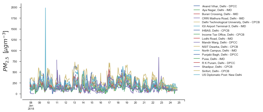
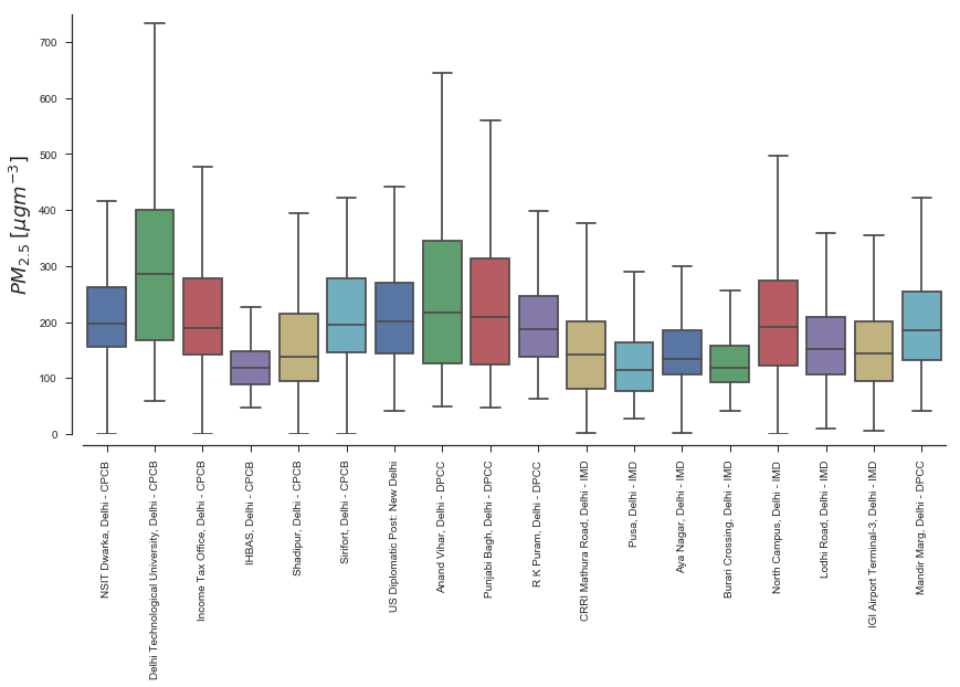
Don’t worry too much about how ugly and uninteresting the plot above is…we’ll take care of that in the next tutorial! Let’s go ahead and look at the distribution of \(PM_{2.5}\) values seen in Delhi by various sensors. This is the same data as above, but viewed in a different way.
fig, ax = plt.subplots(1, figsize=(14,7))

ax = sns.boxplot(
    x='location',
    y='value',
    data=res.query("value >= 0.0"),
    fliersize=0,
    palette='deep',
    ax=ax)

ax.set_ylim([0, 750])
ax.set_ylabel("$PM_{2.5}\;[\mu gm^{-3}]$", fontsize=18)
ax.set_xlabel("")

sns.despine(offset=10)

plt.xticks(rotation=90)
plt.show()
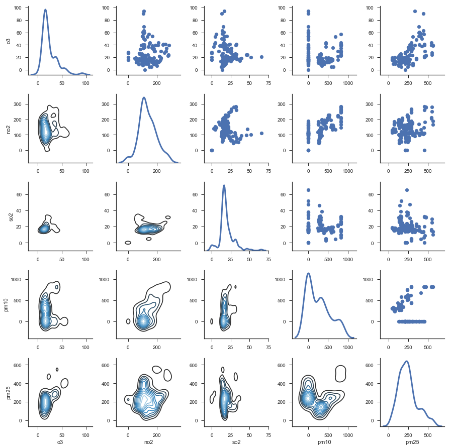
If we remember from above, there was at least one location where many parameters were measured. Let’s go ahead and look at that location and see if there is any correlation among parameters!
res = api.measurements(city='Delhi', location='Anand Vihar', limit=1000, df=True)

# Which params do we have?
res.parameter.unique()
array(['o3', 'no2', 'so2', 'pm10', 'pm25'], dtype=object)
df = pd.DataFrame()

for u in res.parameter.unique():
    _df = res[res['parameter'] == u][['value']]
    _df.columns = [u]

    # Merge the dataframes together
    df = pd.merge(df, _df, left_index=True, right_index=True, how='outer')

# Get rid of rows where not all exist
df.dropna(how='any', inplace=True)

g = sns.PairGrid(df, diag_sharey=False)

g.map_lower(sns.kdeplot, cmap='Blues_d')
g.map_upper(plt.scatter)
g.map_diag(sns.kdeplot, lw=3)

plt.show()
For kicks, let’s go ahead and look at a timeseries of \(SO_2\) data in Hawai’i. Quiz: What do you expect? Did you know that Hawai’i has a huge \(SO_2\) problem?
res = api.measurements(city='Hilo', parameter='so2', limit=10000, df=True)

# Print out the statistics on a per-location basiss
res.groupby(['location'])['value'].describe()
| count | mean | std | min | 25% | 50% | 75% | max | |
|---|---|---|---|---|---|---|---|---|
| location | ||||||||
| Hawaii Volcanoes NP | 355.0 | 0.007392 | 0.035338 | 0.000 | 0.000 | 0.000 | 0.000 | 0.408 |
| Hilo | 438.0 | 0.002486 | 0.004487 | 0.000 | 0.001 | 0.001 | 0.002 | 0.050 |
| Kona | 450.0 | 0.003273 | 0.004264 | 0.001 | 0.001 | 0.002 | 0.004 | 0.039 |
| Ocean View | 455.0 | 0.011490 | 0.021762 | 0.000 | 0.001 | 0.004 | 0.011 | 0.182 |
| Pahala | 422.0 | 0.039166 | 0.070299 | 0.000 | 0.004 | 0.010 | 0.040 | 0.554 |
fig, ax = plt.subplots(1, figsize=(10, 5))

for group, df in res.groupby('location'):
    # Query the data to only get positive values and resample to hourly
    _df = df.query("value >= 0.0").resample('6h').mean()

    # Convert from ppm to ppb
    _df['value'] *= 1e3

    # Multiply the value by 1000 to get from ppm to ppb
    _df.value.plot(ax=ax, label=group)

ax.legend(loc='best')
ax.set_ylabel("$SO_2 \; [ppb]$", fontsize=18)
ax.set_xlabel("")

sns.despine(offset=5)

plt.show()
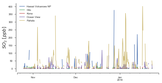
NOTE: These values are for 6h means. The local readings can actually get much, much higher (>5 ppm!) when looking at 1min data.